JaxSim as a hardware-accelerated parallel physics engine-advanced usage#
JaxSim is developed to optimize synthetic data generation by sampling trajectories using hardware accelerators such as GPUs and TPUs.
In this notebook, you’ll learn how to use the key APIs to load a simple robot model (a sphere) and simulate multiple trajectories in parallel on GPUs.
Prepare the environment#
# @title Imports and setup
import sys
from IPython.display import clear_output

IS_COLAB = "google.colab" in sys.modules

# Install JAX and Gazebo
if IS_COLAB:
    !{sys.executable} -m pip install --pre -qU jaxsim
    !apt install -qq lsb-release wget gnupg
    !wget https://packages.osrfoundation.org/gazebo.gpg -O /usr/share/keyrings/pkgs-osrf-archive-keyring.gpg
    !echo "deb [arch=$(dpkg --print-architecture) signed-by=/usr/share/keyrings/pkgs-osrf-archive-keyring.gpg] http://packages.osrfoundation.org/gazebo/ubuntu-stable $(lsb_release -cs) main" | sudo tee /etc/apt/sources.list.d/gazebo-stable.list > /dev/null
    !apt -qq update
    !apt install -qq --no-install-recommends libsdformat13 gz-tools2

    clear_output()

# Set environment variable to avoid GPU out of memory errors
%env XLA_PYTHON_CLIENT_MEM_PREALLOCATE=false

# ================
# Notebook imports
# ================

import os

os.environ["MUJOCO_GL"] = "osmesa"

import jax

import jax.numpy as jnp
import jaxsim.api as js
import rod
from jaxsim import logging
from rod.builder.primitives import SphereBuilder

logging.set_logging_level(logging.LoggingLevel.WARNING)
print(f"Running on {jax.devices()}")
env: XLA_PYTHON_CLIENT_MEM_PREALLOCATE=false
Running on [CpuDevice(id=0)]
Prepare the simulation#
JaxSim supports loading robot descriptions from both SDF and URDF files. This is done using the ami-iit/rod library, which processes these formats.
The rod library also allows creating in-memory models that can be serialized to SDF or URDF. We’ll use this functionality to build a sphere model, which will later be used to create the JaxSim model.
# @title Create the model description of a sphere

# Create a SDF model.
# The builder takes care to compute the right inertia tensor for you.
rod_sdf = rod.Sdf(
    version="1.7",
    model=SphereBuilder(radius=0.10, mass=1.0, name="sphere")
    .build_model()
    .add_link()
    .add_inertial()
    .add_visual()
    .add_collision()
    .build(),
)

# Rod allows to update the frames w.r.t. the poses are expressed.
rod_sdf.model.switch_frame_convention(
    frame_convention=rod.FrameConvention.Urdf, explicit_frames=True
)

# Serialize the model to a SDF string.
model_sdf_string = rod_sdf.serialize(pretty=True)
print(model_sdf_string)

# JaxSim currently only supports collisions between points attached to bodies
# and a ground surface modeled as a heightmap sampled from a smooth function.
# While this approach is universal as it applies to generic meshes, the number
# of considered points greatly affects the performance. Spheres, by default,
# are discretized with 250 points. It's too much for this simple example.
# This number can be decreased with the following environment variable.
os.environ["JAXSIM_COLLISION_SPHERE_POINTS"] = "50"
<?xml version="1.0" encoding="utf-8"?>
<sdf version="1.7">
  <model name="sphere">
    <pose>0.0 0.0 0.0 0.0 0.0 0.0</pose>
    <link name="sphere_link">
      <pose relative_to="__model__">0.0 0.0 0.0 0.0 0.0 0.0</pose>
      <inertial>
        <mass>1.0</mass>
        <inertia>
          <ixx>0.004000000000000001</ixx>
          <iyy>0.004000000000000001</iyy>
          <izz>0.004000000000000001</izz>
          <ixy>0.0</ixy>
          <ixz>0.0</ixz>
          <iyz>0.0</iyz>
        </inertia>
        <pose relative_to="sphere_link">0.0 0.0 0.0 0.0 0.0 0.0</pose>
      </inertial>
      <visual name="sphere_visual">
        <geometry>
          <sphere>
            <radius>0.1</radius>
          </sphere>
        </geometry>
        <pose relative_to="sphere_link">0.0 0.0 0.0 0.0 0.0 0.0</pose>
      </visual>
      <collision name="sphere_collision">
        <geometry>
          <sphere>
            <radius>0.1</radius>
          </sphere>
        </geometry>
        <pose relative_to="sphere_link">0.0 0.0 0.0 0.0 0.0 0.0</pose>
      </collision>
    </link>
  </model>
</sdf>
Create the model and its data#
JAXsim offers a simple functional API in order to interact in a memory-efficient way with the simulation. Four main elements are used to define a simulation:
model: an object that defines the dynamics of the system.data: an object that contains the state of the system.integrator(Optional): an object that defines the integration method.integrator_metadata(Optional): an object that contains the state of the integrator.
The JaxSimModel object contains the simulation time step, the integrator and the contact model.
In this example, we will explicitly pass an integrator class to the model object and we will use the default SoftContacts contact model.
# Create the JaxSim model.
# This is shared among all the parallel instances.
model = js.model.JaxSimModel.build_from_model_description(
    model_description=model_sdf_string,
    time_step=0.001,
)

# Create the data of a single model.
# We will create a vectorized instance later.
data_single = js.data.JaxSimModelData.zero(model=model)
# Initialize the simulated time.
T = jnp.arange(start=0, stop=1.0, step=model.time_step)
Sample a batch of trajectories in parallel#
With the provided resources, you can step through an open-loop trajectory on a single model using jaxsim.api.model.step.
In this notebook, we’ll focus on running parallel steps. We’ll use JAX’s automatic vectorization to apply the step function to batched data.
Note that these parallel simulations are independent — models don’t interact, so there’s no need to avoid initial collisions.
# @title Generate batched initial data

# Create a random JAX key.
key = jax.random.PRNGKey(seed=0)

# Split subkeys for sampling random initial data.
batch_size = 16
row_length = int(jnp.sqrt(batch_size))
row_dist = 0.3 * row_length
key, *subkeys = jax.random.split(key=key, num=batch_size + 1)

# Create the batched data by sampling the height from [0.5, 0.6] meters.
data_batch_t0 = jax.vmap(
    lambda key: js.data.random_model_data(
        model=model,
        key=key,
        base_pos_bounds=([0, 0, 0.3], [0, 0, 1.2]),
        base_vel_lin_bounds=(0, 0),
        base_vel_ang_bounds=(0, 0),
    )
)(jnp.vstack(subkeys))

x, y = jnp.meshgrid(
    jnp.linspace(-row_dist, row_dist, num=row_length),
    jnp.linspace(-row_dist, row_dist, num=row_length),
)
xy_coordinate = jnp.stack([x.flatten(), y.flatten()], axis=-1)

# Reset the x and y position to a grid.
data_batch_t0 = data_batch_t0.replace(
    model=model,
    base_position=data_batch_t0.base_position.at[:, :2].set(xy_coordinate),
)

print("W_p_B(t0)=\n", data_batch_t0.base_position[0:10])
W_p_B(t0)=
 [[-1.2     -1.2      1.00667]
 [-0.4     -1.2      0.83736]
 [ 0.4     -1.2      0.54642]
 [ 1.2     -1.2      0.39748]
 [-1.2     -0.4      0.96483]
 [-0.4     -0.4      0.66458]
 [ 0.4     -0.4      0.93391]
 [ 1.2     -0.4      0.74388]
 [-1.2      0.4      1.01903]
 [-0.4      0.4      0.74109]]
# @title Create parallel step function

import functools
from typing import Any


@jax.jit
def step_single(
    model: js.model.JaxSimModel,
    data: js.data.JaxSimModelData,
) -> tuple[js.data.JaxSimModelData, dict[str, Any]]:

    # Close step over static arguments.
    return js.model.step(
        model=model,
        data=data,
        link_forces=None,
        joint_force_references=None,
    )


@jax.jit
@functools.partial(jax.vmap, in_axes=(None, 0))
def step_parallel(
    model: js.model.JaxSimModel,
    data: js.data.JaxSimModelData,
) -> tuple[js.data.JaxSimModelData, dict[str, Any]]:

    return step_single(
        model=model, data=data
    )


# The first run will be slow since JAX needs to JIT-compile the functions.
_ = step_single(model, data_single)
_ = step_parallel(model, data_batch_t0)

# Benchmark the execution of a single step.
print("\nSingle simulation step:")
%timeit step_single(model, data_single)

# On hardware accelerators, there's a range of batch_size values where
# increasing the number of parallel instances doesn't affect computation time.
# This range depends on the GPU/TPU specifications.
print(f"\nParallel simulation steps (batch_size={batch_size} on {jax.devices()[0]}):")
%timeit step_parallel(model, data_batch_t0)
Single simulation step:
2.51 ms ± 97.7 μs per loop (mean ± std. dev. of 7 runs, 100 loops each)

Parallel simulation steps (batch_size=16 on TFRT_CPU_0):
4.53 ms ± 8.69 μs per loop (mean ± std. dev. of 7 runs, 100 loops each)
# @title Run parallel simulation

data = data_batch_t0
data_trajectory_list = []

for _ in T:

    data = step_parallel(model, data)
    data_trajectory_list.append(data)
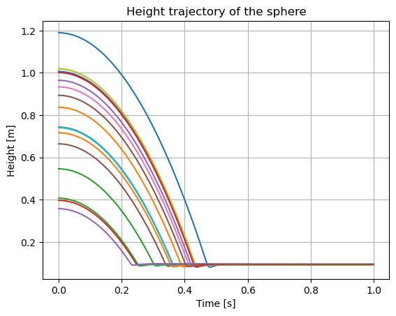
Visualize trajectory#
# Convert a list of PyTrees to a batched PyTree.
# This operation is called 'tree transpose' in JAX.
data_trajectory = jax.tree.map(lambda *leafs: jnp.stack(leafs), *data_trajectory_list)

print(f"W_p_B: shape={data_trajectory.base_position.shape}")
W_p_B: shape=(1000, 16, 3)
import matplotlib.pyplot as plt


plt.plot(T, data_trajectory.base_position[:, :, 2])
plt.grid(True)
plt.xlabel("Time [s]")
plt.ylabel("Height [m]")
plt.title("Height trajectory of the sphere")
plt.show()
import jaxsim.mujoco

mjcf_string, assets = jaxsim.mujoco.ModelToMjcf.convert(
    model.built_from,
    cameras=jaxsim.mujoco.loaders.MujocoCamera.build_from_target_view(
        camera_name="sphere_cam",
        lookat=[0, 0, 0.3],
        distance=4,
        azimuth=150,
        elevation=-10,
    ),
)

# Create a helper for each parallel instance.
mj_model_helpers = [
    jaxsim.mujoco.MujocoModelHelper.build_from_xml(
        mjcf_description=mjcf_string, assets=assets
    )
    for _ in range(batch_size)
]

# Create the video recorder.
recorder = jaxsim.mujoco.MujocoVideoRecorder(
    model=mj_model_helpers[0].model,
    data=[helper.data for helper in mj_model_helpers],
    fps=int(1 / model.time_step),
    width=320 * 2,
    height=240 * 2,
)

for data_t in data_trajectory_list:

    for helper, base_position, base_quaternion, joint_position in zip(
        mj_model_helpers,
        data_t.base_position,
        data_t.base_orientation,
        data_t.joint_positions,
        strict=True,
    ):
        helper.set_base_position(position=base_position)
        helper.set_base_orientation(orientation=base_quaternion)

        if model.dofs() > 0:
            helper.set_joint_positions(
                positions=joint_position, joint_names=model.joint_names()
            )

    # Record a new video frame.
    recorder.record_frame(camera_name="sphere_cam")
import mediapy as media

media.show_video(recorder.frames, fps=recorder.fps)